Paper Note: VITS
Abstract
VITS: Conditional Variational Autoencoder with Adversarial Learning for End-to-End Text-to-Speech [1].
VITS aims to improve the performance of ene-to-end (single stage) TTS model, so that the quality of synthesized speech meets or exceeds that of two-stage systems.This paper is published at ICML 2021.
This note provides explanation and summary of VITS.
1. Introduction
Traditional TTS model is a two-stage system: 1. text -> middle feature (mel-spectrograms, linguistic features, etc.); 2. middle feature -> raw waveforms. The models at each of the two-stage pipelines are developed independently in the past [2]. Thus, there is a gap between the stages, which can result in high training costs and slow inference. Besides, the quality of synthesized speech from two-stage systems might not high enough (Note: in second-stage system, for example, spectrogram-to-waveform model is trained through real spectrogram. The quality of the spectrogram generated in the first-stage system might not be up to the real spectrogram's, which leads to degradation of the speech quality while inference).
The overall architecture of the model consists of a posterior encoder, a prior encoder, a decoder, a discriminator, and a stochastic duration predictor. The posterior encoder and discriminator are only used during training and are not involved in inference. VITS introduces four modules to generate more natural audio:
- Variational autoencoder (VAE)
- Normalizing flows (improve quality of speech)
- GAN (assist training)
- Stochastic duration predictor (one-to-many, diverse rhythms)
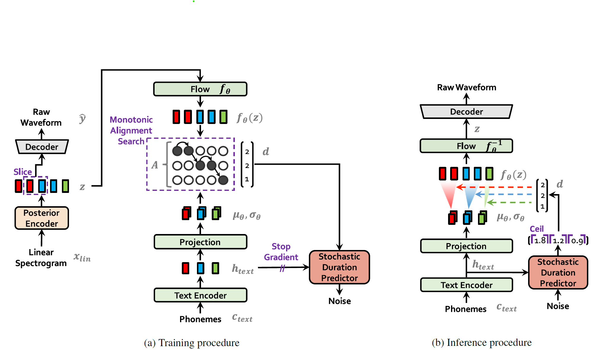
Fig.1 (a) is the training stage. Fig.1 (b) is the inference stage.
Training stage
Text encoder: The transformer-based text encoder, which encodes isolated text into features with contextual information.
Prior encoder: Take the text (output from text encoder) and speaker embedding as input to get the prior distribution $z$.
Posterior encoder: Input: linear spectrogram and speaker embedding.
Stochastic Duration Predictor: To predict a distribution of the duration for a single phoneme.
Note that, since the prior encoder takes $c_{text}$ and speaker embedding as input while the posterior encoder takes the linear spectrogram and speaker embedding as input, the length of outputs from them would not be the same. Thus, we need to apply an alignment processing via monotonic alignment search.
2. Method
2.1 Variational inference
2.1.1 Overview
VITS can be expressed as a conditional VAE. The core formula is then,
$$
\log p_{\theta}(x|\theta) \geqslant \mathbb{E}_{q_\phi(z|x)}[\text{log}p_\theta(x|z) - \text{log}\frac{q_\phi(z|x)}{p_\theta(z|c)}]\tag{2.1}
$$
where $c$ denotes the condition, that is, the text, $x$ can be considered as the generated waveform;
$p_{\theta}(x|\theta)$ denotes the probability that we need to maximize, with the model parameters $\theta$.
It is difficult to maximize the this model directly. Thus, we maximize its variational lower bound, AKA evidence lower bound (ELBO). Since it involves conditions, we use the conditional variational lower bound here;
$z$ denotes the latent variable;
$p_\theta(z|c)$ represents the prior distribution of latent variables given conditions;
$p_{\theta}(x|z)$ is the likelihood of $x$, can be understood as the probability of obtaining $x$ given $z$, that is, the Decoder. (In other words, the target waveform $x$ is reconstructed through the latent variable $z$);
$q_\phi(z|x)$ is the approximate posterior distribution of $x$;
$\text{log}\frac{q_\phi(z|x)}{p_\theta(z|c)}$ is the KL divergence: $\text{log}q_\phi(z|x) - \text{log}{p_\theta(z|c)}$. Here, $q_\phi(z|x)$ denotes the posterior distribution of $z$ (latent variable) given $x$ (predicted output waveform) predicted by the model $\phi$; $p_\theta(z|c)$ denotes the prior distribution of $z$ give $c$ (the input text).
In general, to maximize the lower bound, there are two steps. First, we need to maximize the output from decoder $\text{log}~p_\theta(x|z)$, that is, the model $\theta$ needs to predict output $x$ well when given $z$. Second, we need to minimize the KL divergence, which is the distance between the posterior distribution and the prior distribution. Simply, the goal is to minimize the distance between the distribution of $z$ predicted by model $\phi$ given $x$ and the distribution of $z$ predicted by model $\theta$ given $c$.
A detailed introduction to Conditional VAE can be found in this article.
In Eq. (2.1), $x$ denotes linear spectrogram of the audio, $c$ denotes the text and alignment, $z$ denotes latent variable. Alignment information is a matrix, which with shape of $\text{[|text|, |z|]}$.
2.1.2 Reconstruction Loss
The use mel-spectrogram as the reconstruct target $x_{mel}$.
- Upsampling the latent variables $z$ to the waveform domain $\hat y$
- Transform $\hat y$ to mel-spectrogram $\hat{x}_{mel}$
- Calculate the $L_1$ Loss
$$
L_{recon} = ||x_{mel} - \hat x_{mel}||_1 \tag{2.2}
$$
The reason of using mel-spectrogram instead of waveform is to improve the perceptual quality.
2.1.3 KL Divergence
The input condition of the prior encoder $c$ is composed of phonemes $c_{text}$ (text -> pinyin / phonemes -> Transformer Encoder -> $c_{text}$) extracted from text and an alignment $A$ between phonemes and latent variables.
The alignment matrix $A$ is a hard monotonic attention matrix.
Monotonic: The current spectrum corresponds to the current or following word or text, but not to the previous one.
Hard: Single spectrum corresponds to single word or text, not one to many.
So the shape of alignment matrix would be $|c_{text}| \times |z|$ dimensions representing how long each input phoneme expands to be time-aligned with the target speech.
However, the training set only provides the text and the waveform, not include the alignment information. So we must estimate the alignment at each training iteration.
To provide high-resolution information for the posterior encoder, we use the linear-scale spectrogram of target speech $x_{lin}$ rather than mel-spectrogram. The KL divergence is then:
$$
\displaylines{L_{kl} = \log q_\phi(z|x_{lin}) - \log p_\theta(z|c_{text}, A),
\\ z \sim q_\phi(z|x_{lin}) = N(z;\mu_\phi(x_{lin}), \sigma_\phi(x_{lin}))} \tag{2.3}
$$
Note that the $z$ is sampled from the posterior distribution, which is a Gaussian distribution.
In order to increase the expressiveness of the prior distribution to generate more realistic sample, we introduce normalizing flow $f_\theta$, which allows simple distributions to be reversibly transformed into more complex distributions according to the pattern of change of the variable. Then,
$$
\displaylines{p_\theta(z|c) = N(f_\theta(z);\mu_\theta(c), \sigma_\theta(c))|\det\frac{\partial f_\theta(z)}{\partial z}|,
\\ c = [c_{text}, A]} \tag{2.4}
$$
Why normalizing flow? Pleas reference to this article.
2.2 Alignment Estimation
2.2.1 Monotonic Alignment Search
To estimate the alignment matrix $A$ between input text and target speech, we adopt MAS, a method to search an alignment that maximizes the likelihood of data parameterized by a normalizing flow $f$:
$$
\displaylines{A = \text{arg max}_{\hat A} \log p(x|c_{text}, \hat{A})
\\ = \text{arg max}_{\hat A} log N(f(x); \mu(c_{text}, \hat{A}), \sigma(c_{text}, \hat{A}))} \tag{2.5}
$$
Note that the alignments must be monotonic and non-skipping. Because the objective is the ELBO, instead of the exact log-likelihood. MAS need to redefine to find an alignment that maximizes the ELBO, which reduces to finding an alignment that maximizes the log-likelihood of the latent variables $z$:
$$
\displaylines{\text{arg max}_{\hat A} \log p_\theta(x_{mel}|z) - \log\frac{q_\phi(z|x_{lin})}{p_\theta(z|c_{text}, \hat A)}
\\ = \text{arg max}_{\hat A} \log p_\theta(z|c_{text}, \hat A)
\\ = \log N(f_\theta(z); \mu_\theta(c_{text}, \hat A), \sigma_\theta(c_{text}, \hat A))} \tag{2.6}
$$
2.2.2 Duration Prediction from Text
Because the MAS uses the posterior information which cannot be used while inference, we introduce duration prediction. The duration of each input token (world or phoneme) $d_i$ can be calculate by summing all the columns in each row of the estimated alignment $\sum_j A_{i, j}$ (where the $i$ the input token and the $j$ the spectrogram). The duration could be used to train a deterministic duration predictor. To make the model much more expressive, the duration predictor is designed to be stochastic, that is, a duration distribution of given phonemes instead of a fixed duration.
The stochastic duration predictor is a flow-based generative model. We introduce two random variables $u$ and $v$, which have the same time resolution and dimension as that of the duration sequence $d$, for variational dequantization and variational data augmentation.
2.3 Adversarial Training
Using traditional loss function (like L1 loss between the generated waveform and the ground truth) or reconstruct loss (like MSE loss between the generated mel spectrogram and the ground truth's) to train the model, the generated wave would be unnatural.
Thus, we add a discriminator $D$ to fix this problem. The decoder is the generator $G$. So, the loss functions are:
$$
L_{\text{adv}}(D) = \mathbb{E}_{(y, z)}[(D(y) - 1)^ 2 + (D(G(z)))^2] \tag{2.7}
$$
$$
L_{\text{adv}}(G) = \mathbb{E}[(D(G(z)) - 1)^2] \tag{2.8}
$$
$$
L_{\text{fm}} = \mathbb{E}_{(y,z)}[\sum _{l=1}^T\frac{1}{N_l}||D^l(y) - D^l(G(z))||_1] \tag{2.9}
$$
In formula 2.9, $T$ denotes the total number of layers in the discriminator and $D^l$ outputs the feature map of the $l$-th layer of the discriminator with $N_l$ number of features. The feature mapping loss can be seen as reconstruction loss that is measured in the hidden layers of the discriminator suggested as an alternative to the element-wise reconstruction loss of VAEs.
2.4 Final Loss
$$
L_{\text{vae}} = L_{\text{recon}} + L_{\text{kl}} + L_{\text{dur}} + L_{\text{adv}}(G) + L_{\text{fm}}(G) \tag{2.10}
$$
$L_{\text{recon}}$ is the mel loss.
2.5 Model Architecture
There are four module in the model:
- Posterior Encoder: use the linear spectrogram as input
- prior Encoder: use the text and speaker information as input
- Decoder: reconstruct the latent variable $z$ to waveform
- Discriminator: for GAN, use waveform as input
- Stochastic Duration Predictor
Note that the posterior encoder and the discriminator only be used in training stage.
2.5.1 Posterior Encoder
Non-causal WaveNet residual blocks, consists of layers of dilated convolutions with a gated activation unit and skip connection. Then there will be a linear projection to get the mean and variance of the normal posterior distribution.
For multi-speaker case, the speaker embedding should be added as condition.
2.5.2 Prior Encoder
Prior encoder consists of two modules.
Text encoder. Using transformer encoder with relative positional embedding to encode the input text to get $c_\text{text}$. We can obtain the hidden representation $h_\text{text}$ from $c_\text{text}$. Then a linear projection would be used to calculate the mean and variance of the prior distribution.
Normalizing Flow. $f_\theta$ would be used to expand the expressiveness of the model. The flow is a stack of affine coupling layers.
2.5.3 Decoder
The decoder is like the traditional vocoder. In detail, decoder reconstruct the waveform from the latent variable $z$ instead of the spectrogram as the traditional vocoder.
2.5.4 Discriminator
HiFi-GAN
Stochastic Duration Predictor
A stack of residual blocks with dilated and depth-separable convolutional layers.
Normalizing Flow.
3. Code Explanation
https://github.com/jaywalnut310/vits
3.x Stochastic Duration Predictor
3.x.1 Definition
3.x.2 Principle
Variational Dequantization
Each word or text maps to specified integer numbers of spectrogram. So the distribution of duration is discrete. To model this distribution, we can use a continuous distribution to replace it to derive the lower bound of the target distribution log-likelihood. This lower bound is defined as:
$$
\mathbb{E}_{u\sim q(u|x)} \log p(x+u) - \log q(u|x) \tag{3.1}
$$
where, the $x$ is the target distribution, $q(u|x)$ the posterior distribution, $p(x+u)$ the model distribution.
- Generally, $q(u|x)$ is a conditional flow model, $u=q_x(\text{eps})$, $\text{eps}$ is a noise randomly sample from the Gaussian Distribution. So, we can get $\log q(u|x) = \log(\text{eps}) + log |\det [\frac{\partial q^{-1}}{\partial u}]| = \log(\text{eps}) - log |\det [\frac{\partial q}{\partial \text{eps}}]|$.
Variational Data Augmentation
Reference
[1] Kim J, Kong J, Son J. Conditional variational autoencoder with adversarial learning for end-to-end text-to-speech[C]//ICML. PMLR, 2021: 5530-5540.
[2] Oord A, Dieleman S, Zen H, et al. Wavenet: A generative model for raw audio[J]. arXiv preprint arXiv:1609.03499, 2016.
[3]