Variational Auto-Encoders
Abstract
Variational Auto-Encoders (VAEs) are a type of generative model that combines probabilistic graphical models and neural networks. They are capable of learning latent variable representations of data and generating new data samples given some input data. VAEs approximate the log-likelihood by maximizing the variational lower bound, thus avoiding the direct maximization of potentially intractable objective functions.
1. Introduction
In general, for VAE, a low-dimensional space $z$ can be mapped to high-dimensional space true data, like photos, songs.
1.1 Compared with GAN
VAE is similar to GAN. Both of them are to generate (new) data. In GAN, the point is to derive models that approximate the input distribution. In VAE, the focus is on how to model the input distribution in a decouplable continuous latent space.
VAE take random sample of a specific distribution as input and can generate corresponding data, which is similar to GAN's goal in this respect. However, VAE doesn't need discriminator, but encoder to estimate the specific distribution.
For example, given a serious of photos of cats, we hope the model can generate a new cat photo by input a $n$-dimensional random vector. For GAN, the model does not need to understand the relationship between the cat and the $n$-dimension random vector, but directly fits the distribution of the cat photos with respect to the $n$-dimensional vector by means of adversarial learning.
On the contrary, for VAE, the $n$-dimensional vector represents $n$ invisible factors that determine what the final cat face will look like. There will be a distribution generated corresponding to each factor. Sampling from these distributions and relationships, the model can recover a cat face through a deep neural network.
1.2 Compared with Auto-Encoder
In AE, the model take a data as input and generate a new data same as input data. But in general, the goal is that the generated data is a little bit different from the input, which means that the model need to take random vector as input and is able to learn the stylised features of the generated data.
The architecture of VAE is similar to AE's, which is composed of Encoder (aka recognition / inference module) and Decoder (aka generative module). Both VAE and AE try to learn latent vector and reconstruct data at the same time. The difference is that, compared with AE, the latent space of VAE is continuous, and the decoder itself is used as generative model. VAE introduces variational approach based on AE.
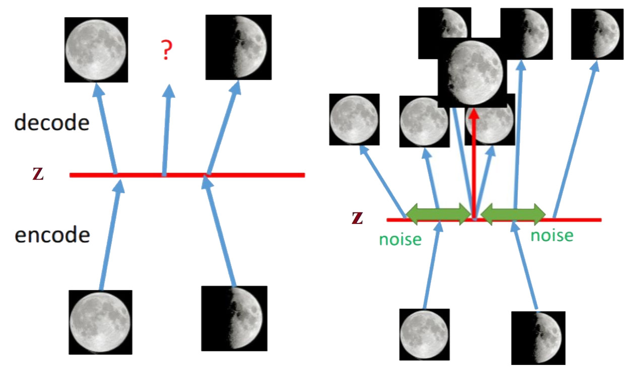
AE is an unsupervised algorithm. The key method is that input feature $x$ can be abstracted as hidden feature $z$, and then $z$ can be predicted or reconstructed as output $\hat{x}$ through decoder. Generally, encoder and decoder could be CNN / RNN / LSTM, etc. The goal of AE is to extract abstract features $z$, that is minimizing the loss function $L(x, \hat{x})$, like:
$$
\displaylines{L(x, \hat{x}) = \sum^n_{i=1}||x_i - x||^2 \\=\sum^n_{i=1}||x_i - g(f(x_i))||^2} \tag{1.1}
$$
where $f(\cdot)$ denotes the encoder, $g(\cdot)$ denotes the decoder, $x_i$ contains $n$ features, i.e., $x_i \in \mathbb{R}^n$.
2 VAE
2.1 Principle of VAE
Suppose the dataset is $X = {x^{(i)}}^N_{i=1}$ is sampled from continuous or discrete variable $x$.
Suppose the data is generated by a random process and contains a invisible continuous random hidden variable $z$. There are two steps to generate:
- $z^{(i)}$ is generated by sampling from prior distribution $P_\theta(z)$;
- Generate $x^{(i)}$ from conditional probability distribution. (This process is hard to compute.)
The original VAE does not model $p_\theta{z}$, instead, model $Q_\phi(z|x)$ to approximate $P_\theta{z|x}$. The author recognizes the process of using $Q_\phi(z|x)$ as Encoder, that is, it can learn a corresponding hidden distribution $z$ for each sample $x$ (note that each sample can be learnt its hidden distribution $z$); the process of using $P_\theta{z|x}$ can be seen as Decoder to generate new data.
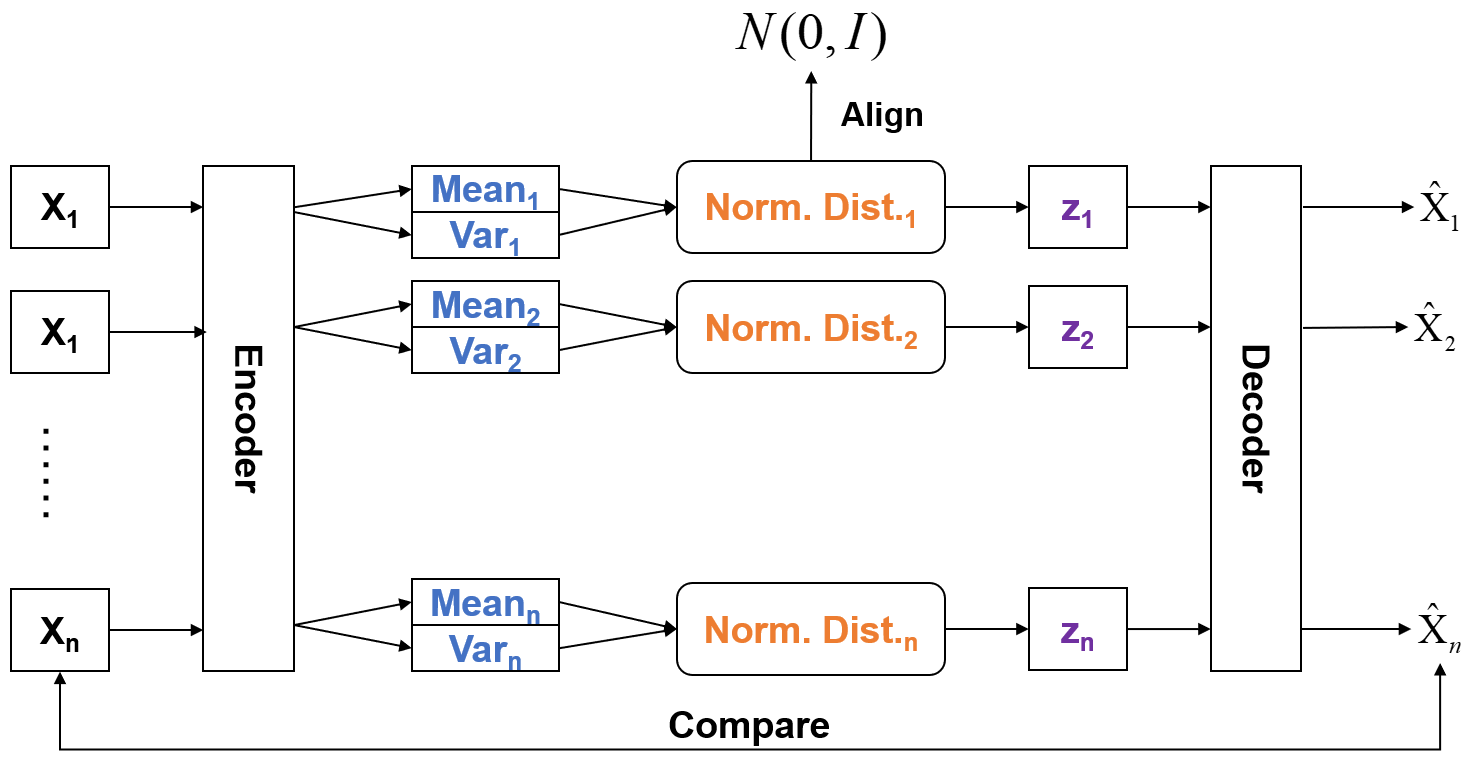
The architecture of VAE is shown in Figure 2. VAE will match a Gaussian Distribution for each sample $X$. Hidden variable $Z$ is sampled from Gaussian Distribution. For $K$ samples, suppose the Gaussian Distribution for each sample was $\mathcal{N}(\mu_k, \sigma^2_k)$. The key is how to approximate those distributions. VAE uses two neural networks to approximate the mean and the variance, that is, $\mu_k=f_1(X_k)$ and $\text{log}\sigma^2_k = f_2(X_k)$. In order to make each Gaussian Distribution as close as possible to the Standard Gaussian Distribution, KL divergence is used to calculate the loss.
2.2 Original VAE
Suppose the distribution of original sample data $x$ is,
$$
x \sim P_\theta(x) \tag{1.2}
$$
where, $\theta$ denotes the model's parameters.
Here, we consider that $x$ is generated by hidden variable $z$. $z$ represents an encoding of specific attributes that can be obtained or inferred from input data.
For example, in human face image generation, attributes might be eyes, nose, mouth, hair style, etc.
In fact, $P_\theta(x, z)$ denotes the distribution of the input data and its attributes. To obtain $P_\theta(x)$, we can
$$
P_\theta(x) = \int P_\theta(x, z), dz \tag{1.3}
$$
In Eq. 1.3, the problem is that it has no analytical form or valid estimator. Therefor, optimizing it via NN is not feasible. According to Bayes' theorem, we can convert Eq. 1.3 to
$$
P_\theta(x) = \int P_\theta(x|z)P(z), dz \tag{1.4}
$$
Here, $P(z)$ is the prior distribution of $z$. When $z$ is discrete and $P_\theta{x|z}$ is Gaussian Distribution, $P_\theta(x)$ is Gaussian Mixture Distribution; When $z$ is continuous, the $P_\theta(x)$ unpredictable. What’s more, for most of $z$, $P_\theta(x|z)$ is equal to $0$ because the sample space of $z$ is too large. Thus, we need to reduce the sample space (or increase the probability of generating $x$ from $z$), and it is simpler to compute the expectation when $z \sim Q(z|X)$.
In more detail, suppose that $z \sim N(0, 1)$, prior distribution $P(x|z)$ is Gaussian Distribution, that is, $x|z \sim N(\mu(z), \sigma(z))$. $\mu(z)$ and $\sigma(z)$ are the functions denote the mean and variance of Gaussian Distribution corresponding to $z$. Then $P(x)$ is the cumulative of all Gaussian Distributions over the domain of integration. $P(z)$ is known, while $P(x|z)$ is unknown. So the fact is that to figure out the function $\mu$ and the function $\sigma$. The original target is solve $P(x)$, and the larger $P(x)$ the better. It is equivalent to solving for the maximum log-likelihood with respect to $x$,
$$
L=\sum_x \text{log} P(x) \tag{1.5}
$$
To process $P(z|x)$ more easier, VAE introduces Variational Inference (Encoder):
$$
Q(z|x) \approx P(z|x) \tag{1.6}
$$
According to Bayes' theorem,
$$
\displaylines{\text{log} P(x) = \int_Z P(z)P(x|z)dz \\ = \int_Z Q(z|x)\text{log}(\frac{P(x, z)}{P(z|x)})dz
\\=\int_Z Q(z|x) \text{log}(\frac{P(x, z)}{Q(z|x)}\frac{Q(z|x)}{P(z|x)})dz
\\=\int_Z Q(z|x)\text{log}(\frac{P(x, z)}{Q(z|x)})dz + \int_Z Q(z|x)\text{log}(\frac{Q(z|x)}{P(z|x)})dz
\\=\int_Z Q(z|x)\text{log}(\frac{P(x|z)P(z)}{Q(z|x)})dz + \int_Z Q(z|x)\text{log}(\frac{Q(z|x)}{P(z|x)})dz} \tag{1.7}
$$
In Eq. 1.7, we can find that $\int_Z Q(z|x)\text{log}(\frac{Q(z|x)}{P(z|x)})dz$ is the KL divergence between $P$ and $Q$, that is, $\text{KL}(Q(z|x)||P(z|x))$. KL divergence is greater than or equal to $0$, so the Eq. 1.7 can be written as,
$$
\text{log}P(x) \geq \int_Z Q(z|x)\text{log}(\frac{P(x|z)P(z)}{Q(z|x)})dz \tag{1.8}
$$
and,
$$
\text{log}P(x) = L_b + \text{KL}(Q(z|x)||P(z|x)) \tag{1.9}
$$
where, $L_b = \int_Z Q(z|x)\text{log}(\frac{P(x|z)P(z)}{Q(z|x)})dz$ is the Evidence Lower Bound (ELBO). The goal is to maximize $L_b$.
Note: Posterior distribution $P(z|x)$ is intractable, so we need to approximate it using $Q(z|x)$. Firstly, $Q(z|x)$ has no relation to $\text{log}P(z|x)$. When adjust $Q(z|x)$ there will be no influence on $L_P$. Thus, when fix $P(x|z)$, maximizing $L_b$ by adjusting $Q(z|x)$, the $KL$ will be smaller. When $Q(z|x)$ approximate posterior distribution $P(z|x)$, $\text{KL} \to 0$. As a result, maximizing $\text{log}P(x)$ equals to maximizing $L_b$.
$$
\displaylines{L_b = \int_Z Q(z|x)\text{log}(\frac{P(x|z)P(z)}{Q(z|x)})dz
\\ = \int_Z Q(z|x)\text{log}(\frac{P(z)}{Q(z|x)})dz + \int_Z Q(z|x)\text{log}P(x|z)dz
\\ = - \text{KL}(Q(z|x)||P(z)) + \int_Z Q(z|x)\text{log}P(x|z)dz
\\ = - \text{KL}(Q(z|x)||P(z)) + E_{Q(z|x)}[\text{log}P(x|z)]} \tag{1.10}
$$
From Eq.10, maximizing $L_b$ means to minimize $\text{KL}(Q(z|x)||P(z))$ and maximize $E_{Q(z|x)}[\text{log}P(x|z)]$.
2.2.1 Maximizing $L_b$
First of all, we need to minimize $\text{KL}(Q(z|x)||P(z))$. We have assumed that $P(z) \sim \mathcal{N}(0, 1)$, and $Q(z|x) \sim \mathcal{N}(\mu, \sigma^2)$, so,
$$
\displaylines{\text{KL}(Q(z|x) || P(z)) = \text{KL}(\mathcal{N}(\mu, \sigma^2) || \mathcal{N}(0, 1))
\\ = \int \frac{1}{\sqrt{2\pi\sigma^2}}e^{\frac{-(x-\mu)^2}{2\sigma^2}}(\text{log}\frac{e^{\frac{-(x-\mu)^2}{2\sigma^2}}/\sqrt{2\pi\sigma^2}}{e^{\frac{-x^2}{2}}/\sqrt{2\pi}})dx
\\ = \frac{1}{2} \frac{1}{\sqrt{2\pi\sigma^2}}\int e^{\frac{-(x-\mu)^2}{2\sigma^2}}(-\text{log} \sigma^2 + x^2 - \frac{(x-\mu)^2}{\sigma^2})dx
\\ = \frac{1}{2} \int \frac{1}{\sqrt{2\pi\sigma^2}} e^{\frac{-(x-\mu)^2}{2\sigma^2}}(-\text{log} \sigma^2 + x^2 - \frac{(x-\mu)^2}{\sigma^2})dx
\\ = \frac{1}{2} (-\text{log} \sigma^2 + \mu^2 + \sigma^2 - 1)} \tag{1.11}
$$
Second, we need to maximize the $E_{Q(z|x)}[\text{log}P(x|z)]$.
- It means that the value of output from Decoder $P(x|z)$ will be as higher as possible given the Encoder $Q(z|x)$ output.
- First, using the Encoder NN to calculate the mean and var., sample $z$ from it. This procession is $Q(z|x)$.
- Second, using the $N$ of Decoder to calculate the mean and var. of $z$, making the mean (or even var.) to much approximate $x$, that is the probability of generating $x$ will be bigger, which is maximizing $\log P(x|z)$.
2.2.2 Reparametrizing
Sampling $z$ from $\mathcal N(\mu, \sigma^2)$ equals to sampling $\epsilon$ from $\mathcal N(0, 1)$ and applying $z=\mu + \epsilon * \sigma$. The reason is that sampling procession is non-derivable but the result.
3 VAE & Neural Network
3.1 Intuition and Understanding of VAE
- The goal of VAE is to get smooth latent space.
- Variational Inference provides a loss function for VAE to maximize ELBO
3.2 Using Neural Network to Build VAE
- Using two neural network “functions” to approximate and synthesis the probability distribution of $p(z|x)$ and $p(x|z)$, and guarantee that both $p(z)$ and $p(z|x)$ are smooth.
Assume that $p(z)$ is a standard normal distribution,
$$
p(z) \sim \mathcal{N}(0, I) \tag{3.1}
$$
$$
q_\theta(z|x) \sim \mathcal{N}(g(x), h(x)),~~g \in G~~~h\in H \tag{3.2}
$$
$$
p_\phi(x|z) \sim \mathcal{N}(f(z), cI),~~f\in F~~~c>0 \tag{3.3}
$$
where, $g(\cdot)$, $h(\cdot)$, and $f(\cdot)$ are the neural network functions.
Note that,
$$
p(z|x) = \frac{p(x|z)p(z)}{p(x)} = \frac{p(x|z)p(z)}{\int p(x|u)p(u)du} \tag{3.4}
$$
Why we can make these assumptions directly?
There are lots of benefits to use Gaussian Distribution:
- Easy to sample datapoint
- Easy to calculate KL divergence
- Satisfies Central Limit Theorem
- The space is smooth
So, the goal is then,
$$
(f^*, g^*, h^*) = \text{arg max}_{(f, g, h) \in F\times G\times H}(\mathbb E_{z\sim q_x}(-\frac{||x-f(z)||^2}{2c}) - \text{KL}(q_x(z), p(z))) \tag{3.5}
$$
Then the loss function is,
$$
\displaylines{\text{Loss} = C||x-\hat{x}||^2 + \text{KL}[N(\mu_x, \sigma_x), N(0,I)]
\\ = C||x-f(z)||^2 + \text{KL}[N(g(x), h(x)), N(0,I)]} \tag{3.6}
$$
Acknowledgement
This note is inspired by Canglan's site.