Normalizing Flow
Abstract
Normalizing flow can convert simple probability densities (e.g. Gaussian Distribution) into some complex form of distribution. It can be used in generative model, reinforcement learning, variational inference, and so on. Flow means that the data “flow” through a series of bijection (invertible mapping) to map to the appropriate representation space. Normalizing means that the variables in the representation space integrate to $1$, satisfying the definition of the probability distribution function.
1 Prior Knowledge
1.1 Overview of Normalizing Flow
In AIGC or GenAI, the goal is generate a result (photo, audio, text, and so on) by giving a condition. The result probably not have seen before and partial random. And the result must be reasonable, that is the latent space is smooth or regularized, basically.
To solve this problem, NF is a useful method.
When we use probabilistic generative model (PGM), assume that there is a true probability distribution (photo, audio, text, and so on) in the world. The PGM is the true probability distribution. We need to figure out the PGM, there are two goals,
- Sampling: get a new data randomly
- Evaluation: calculate the probability of a sample
Evaluation
The Evaluation often be used as a prior condition. For example, when we reconstruct a piece of audio, the probability of this audio “happening / existing” is higher in the real world, the higher the probability that this audio we generate is “correct”.
1.1.1 Principal of Flow
Sampling
Assume that there is a function $f(\cdot)$ and a latent space $z$. We sample a point from $z$ randomly, then apply $f^{-1}(z)$, we would get a target photo.
Evaluation
Assume that there is a photo $x$, we apply $f(x)$, we would get a point located on a simple distribution like Gaussian Distribution, then we can calculate the true probability of the point presenting.
Moving forward, we approximate the true distribution via Change of Variables.
$$
p_X(x) = p_Z(f(x))|\det Df(x)|,~~Z=f(x),~ Df(x)\text{ is Jacobian of}~f(X) \tag{1.1}
$$
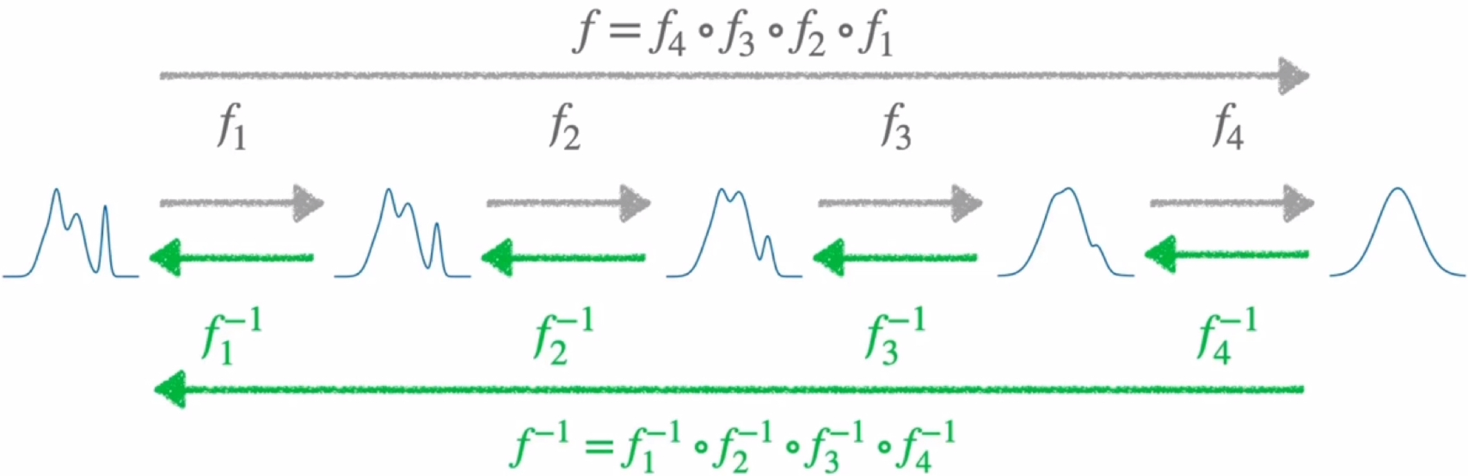
From Fig.1, a complex probability distribution can be transform to a simple probability distribution through a series of transform functions $f_n$. The correspond simple probability distribution can be transform back to the complex probability through the inverse function $f_n^{-1}$. That is Change of Variables.
There is a natural benefit of Flow, that is make sure that the latent space is smooth. Because the Gaussian Distribution is smooth at the very beginning, if only apply transformation or mapping to it, the result must be smooth (the $f(\cdot)$ has to preserve the smoothness).
1.2 Change of Variable & Linear Algebra & Jacobian Matrix
The essence of Change of Variable is to use new space (simple) to represent / replace old space (complex). However, the density of coordinates will be change by Jacobian, and the corresponding probability distribution would be change. Take an easy example, assumed that there is uniform distribution $X \sim \mathcal{U}(0, 1)$. We perform an affine transformation on $X$ through $f(\cdot)$: $Y = f(X) = 2X +1$. As it is a probability distribution, the integration must be $1$. If we use $Y$ directly, the result will be wrong. So we need to apply a Jacobian Matrix to make sure that.
- So we need to find out a appropriate Transformation Matrix to calculate the Jacobian to make a simple distribution to approximate the probability distribution in real world.
As a result, the $\det |\text{Jacobian}|$ is calculate the influence on the change of area or volume by the change of coordinate.
2 Normalizing Flow & Neural Network
2.1 Flow
What is a flow?
Each Change of Variables is a Flow.
A perfect Flow must be:
- Invertible. Need to make sure to sample and evaluate.
- High expressive. To approximate the real complex probability distribution.
- Easy to calculate Jacobian, and the Jacobian should be const.
Linear flow is a simple linear transformation. It is easy to calculate the Jacobian and inverse function. But the expressiveness is weakness. Even though we perform a series of linear flow on a Gaussian Distribution, it is still a Gaussian Distribution which doesn't approximate the real world distribution.
To fix this problem, we introduce Coupling Flow.
2.2 Coupling Flow
Forward Flow
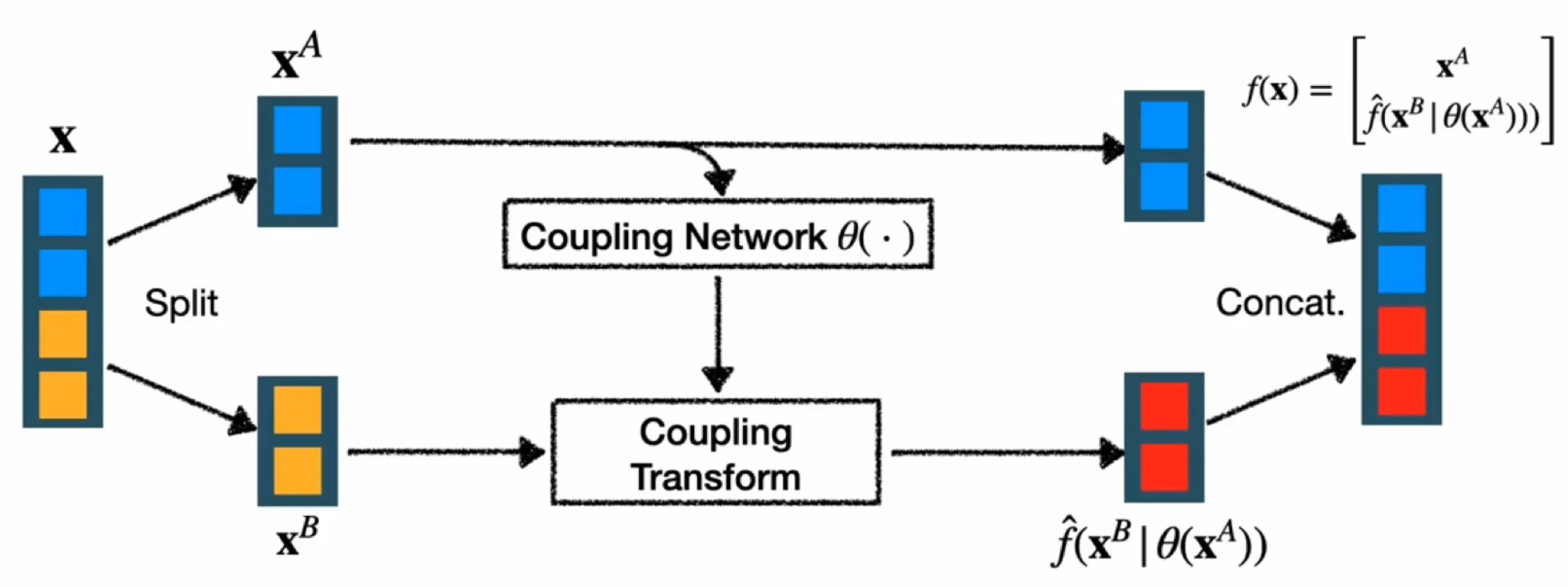
The Jacobian of Coupling Flow is,
$$
\displaylines{Df(x) = \left[
\begin{matrix}
\mathbf{I} & 0 \\
\frac{\partial}{\partial{\mathbf{X}^A}}\hat f (\mathbf{X}^B|\Theta(\mathbf{X}^A)) & D\hat f(\mathbf{X}^B|\theta(\mathbf{X}^A))
\end{matrix}
\right]} \tag{2.1}
$$
$$
\det Df(x) = \det D \hat f (\mathbf{X}^B | \Theta (\mathbf(X)^A)) \tag{2.2}
$$
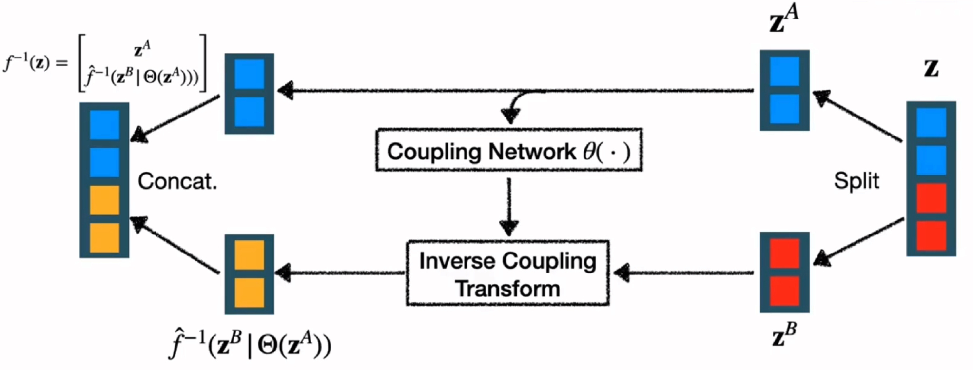
Generally, Coupling Flow uses Linear Function because its $\det|\text{Jacobian}|$ is a constant. The coupling flow is invertible and high non-linear (high expressive).
Of course, when we perform coupling flow, we need to shuffle the input data.